Strategize Bridge Maintenance Effectively
 Source: https://www.webuildvalue.com/wp-content/uploads/2022/02/pittsburgh-bridge-collapse.jpg
Source: https://www.webuildvalue.com/wp-content/uploads/2022/02/pittsburgh-bridge-collapse.jpg
This analysis was originally a project I (Monika Sembiring) did with my friend Tina Feng in our 95885 - Data Science and Big Data class at Carnegie Mellon University.
Prioritizing maintenance for bridges in Allegheny County with these criteria:
Presentation Video Link: https://www.youtube.com/watch?v=z8hvd9e32dk
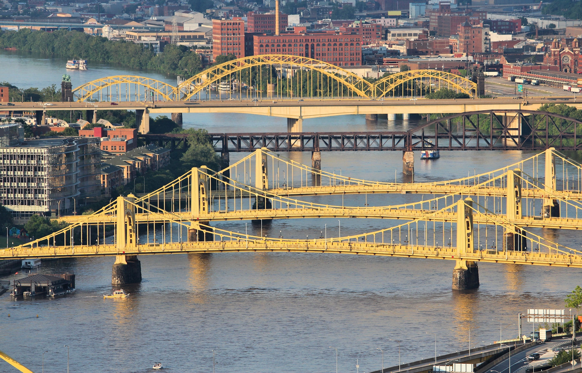
Pittsburgh is the City of Bridges, with nearly 450 bridges. In January 2022, President Biden came to visit Pittsburgh to discuss infrastructure. However, in the morning before his visit, Fern Hollow Bridge collapsed. The detail can be read in this article Pittsburgh Bridge Collapses Hours Before Biden Infrastructure Visit. It was unfortunate that the event might embarrass Pittsburgh a little bit.
However, more than just Pittsburgh's good name and reputation, there is a more significant risk/danger associated with bridge collapse. It is not only dangerous for people who use the bridge when it happens: cars, bicycles, or even pedestrians, but it also might trigger other dangerous things, such as rupturing a gas line.
Fortunately, in the incident of Fern Hollow Bridge, there was no one died. People only had non-life-threatening injuries, and the ruptured gas line was quickly handled. However, what if it happened during busy times when many cars passed the bridge or shutting off the ruptured gas line was difficult? We can imagine how disastrous it will be.
Knowing this condition, we think about whether it is possible to use data to assess the bridge's condition and group them based on its risk/level of collapse. By knowing this information, we can focus on bridges with bad situations and take preventive actions: prepare for better maintenance or even plan to rebuild the bridge. This will also benefit the governments in the long term because they will have a better-allocated infrastructure budget. Preventing the collapse before it happens will save a lot of money because we will not need the money for post-incident handling. This is aligned with the statement from Bridge Master in Spend Less on Keeping Bridges in Good Repair article that bridge repair costs end up being higher than they would have been had the issue been addressed earlier. On the other side, from the perspective of people who live in Pittsburgh, this will be useful for them, too, because it gives them ease of mind when using the bridges themselves because they know the general idea of the bridge they pass every day to do their activities.
In this project, we will analyze bridge data in Allegheny county to achieve these goals:
Since the analysis focus on the bridges in Allegheny county, where Pittsburgh is, this project use combination of the following three datasets:
All datasets above are clean in CSV files. However, we do data preprocessing to ensure the data's quality, select only the features that might be relevant to answer the question we have along with the problem discussed above, and handle multiple columns with missing values. The detail of data preprocessing can be found in the Analysis and Result section.

Source: https://civiljungle.com/wp-content/uploads/2020/11/Substructure-Bridge.png
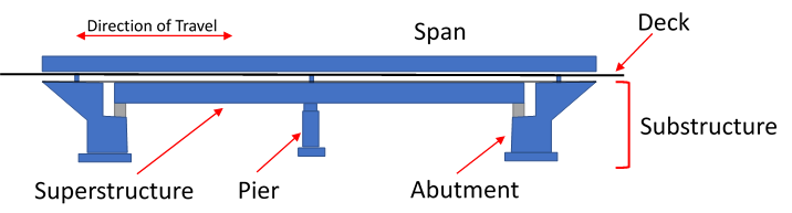
Bridge generally consists of three elements: the substructure, superstructure, and deck of the bridge.
Source: Parts of a Bridge Structure and The Different Components of a Bridge
In terms of structure, there are so many different structures of bridges, but the most common types in the US are these seven types.

Materials for building bridges depend on the type of bridge. However, the most commonly used materials include concrete, steel, stone, and composite.
The process map in Figure 4 is the bridge maintenance reference guide defined by PennDOT. The process is presented as a circle because of the continuity of the bridge inspection/maintenance process, which becomes a series of cycles across time. With this analysis result, we provide added value in the Select Bridge Activities and Maintenance Work Order.

Source: Bridge Maintenance Manual
After exploring the dataset, reading the data dictionary, and studying the bridge features that affect the bridge's condition, we specify the columns that we will use from each of the datasets.
From the main dataset, we choose 15 out of 25 columns because the other columns contain information that is not related to the bridge condition, such as BR Key, County, and Municipality, or they contain only missing values, such as Weight Limit Combination and Weight Limit Single.
From the crash dataset, our main focus is to find the number of times a crash happened on a specific bridge. Therefore we only use latitude, longitude, and flag whether the crash hit the bridge or not.
Lastly, from the more comprehensive bridge dataset, our main focus is to get the latitude and longitude data to join the main dataset and crash dataset. Besides that, we include some other features that affect bridge conditions, such as reconstruction year, eligibility for rehabilitation/replacement, reconstruction cost, and transition rating. Therefore, we only chose ten columns out of 173 columns because the rest of them is not correlated to the bridge condition, have to many missing values, or we are not sure what it represents due to limited explanation in the data dictionary.
The list of columns we used for the analysis can be found in the Analysis and Result section.
To use the data for further analysis, we will preprocess and clean the data first. We will do it with the following steps:
In addition to the above preprocessing steps, we also did Exploratory Data Analysis (EDA) to see data distribution to get insight that might be useful to define the pipeline to standardize data, handle imbalance, and impute missing values.
We build a model for predicting the classification of the bridge condition category, whether it is Good, Bad, or Fair (supervised learning), with the following steps:
After getting the model and performing the analysis, we explore some bridges in Poor condition. We dig deeper in terms of their location, usage, traffic, maintenance cost, and other related variables to produce a framework that can be used to choose the bridges the government should focus the maintenance on. We also showed examples of how to use that framework. With this framework and example's result as a reference, the government can identify in advance the bridges that need different levels of attention and thus maintenance needs to prevent potential future collapse or other accidents.
Number of crashes on bridge calculation: For some bridges that are so close to each other, rounding latitude and longitude coordinates makes them similar in terms of location. Hence when calculating the frequency of crashes on that bridge, we assume that the crash might affect not only the bridge but the area nearby, which is all the bridges close to them, and count effect for all of them.
# import necessary libraries
import pandas as pd
import numpy as np
import altair as alt
import seaborn as sns
pd.set_option('display.max_columns', None)
import warnings
warnings.filterwarnings('ignore')
As mentioned above, we use only some of the columns of the dataset. We only use specific columns related to the bridge's conditions, which helps us with the classification model. A detailed explanation of how we choose particular columns instead of others can be found in the Filter the data columns section.
# column lists for bridge data
main_columns = ['Condition', 'Bridge Id', 'Owner', 'Length (ft)',
'Deck Area (sq ft)', 'Number of Spans', 'Material',
'Structure Type', 'Year Built', 'Deck Condition',
'Superstructure Condition', 'Substructure Condition',
'Culvert Condition', 'Average Daily Traffic',
'Location/Structure Name']
# column list for crash data
crash_columns = ['DEC_LAT', 'DEC_LONG', 'HIT_BRIDGE']
# column lists for comprehensive bridge data
bridge_columns = ['BRIDGE_ID','DEC_LAT', 'DEC_LONG', 'TRANSRATIN', 'TRUCKPCT',
'HBRR_ELIG', 'YEARRECON', 'NBIIMPCOST', 'NBIRWCOST','NBITOTCOST']
# set path for file upload and reading
from google.colab import drive
drive.mount('/content/drive',force_remount=True)
%cd /content/drive/MyDrive/Portfolio/bridge-risk-classification
Mounted at /content/drive /content/drive/MyDrive/Portfolio/bridge-risk-classification
# read the file
df_main = pd.read_excel('data/BridgeConditionReport_County-02_2022-11-13.xlsx',
usecols=main_columns)
df_crash = pd.read_csv('data/crash_2004-2020.csv', usecols=crash_columns)
df_bridge = pd.read_csv('data/Pennsylvania_Bridges.csv', usecols=bridge_columns)
Merging the main and supporting bridge features datasets is simple because we just need to join them on Bridge ID.
# merge the main and bridge dataset based on Bridge ID
df = df_main.merge(df_bridge, how='left',left_on='Bridge Id', right_on='BRIDGE_ID')
# drop duplicates bridge ID column after merge
df = df.drop(['BRIDGE_ID'], axis=1)
When we merge the crash data, we match the crash latitude and longitude with the bridge latitude and longitude by rounding them into two decimals first. Then we count the frequency of crashes on each bridge and merge it into the bridge dataset. We use the assumption mentioned in the Assumption section for the calculation.
# filter only the crash that hit bridge
df_crash = df_crash[df_crash['HIT_BRIDGE'] == 1]
# drop HIT_BRIDGE column
df_crash = df_crash.drop(['HIT_BRIDGE'], axis=1)
# check missing value
pd.concat([df_crash.isna().sum(), df_crash.isna().sum()/len(df_crash)*100], axis=1)
| 0 | 1 | |
|---|---|---|
| DEC_LAT | 45 | 6.072874 |
| DEC_LONG | 45 | 6.072874 |
# since the percentage of missing value is small ~6%,
# we drop the data with missing latitude and longitude
df_crash = df_crash.dropna()
# data from main dataframe to join with the crash data
col = df[['DEC_LAT','DEC_LONG', 'Bridge Id']]
# round the latitude longitude with two decimal places
df_crash = df_crash.round(2)
col = col.round(2)
# merge crash and col to get qty of crash for each bridges
join = pd.merge(df_crash, col,
on = ['DEC_LAT','DEC_LONG'],
how ='left')
We calculate the number of crashes in the bridges by counting the occurrence frequency based on the merge crash and main dataframe we got previously. We then convert the crash calculation back to the dataframe and join it to the main dataframe.
# convert Bridge ID column to list
c = join['Bridge Id'].tolist()
# get frequency of each Bridge ID
from collections import Counter
counts = Counter(c)
# convert freq count result into list
cl = list(counts.items())
# convert frequency into dataframe
crash_count = pd.DataFrame(cl, columns =['Bridge_ID', 'Crash_Count'])
# join the crash data into main dataset
df = df.merge(crash_count, how='left', left_on='Bridge Id', right_on='Bridge_ID')
# replace NaN in HBRR_ELIG column value to Other
df['Crash_Count'] = df['Crash_Count'].fillna(0)
# change the reconstruction age type into integer
df['Crash_Count'] = df['Crash_Count'].astype(int)
# final df shape
df.shape
(1576, 26)
df.head()
| Condition | Bridge Id | Location/Structure Name | Owner | Length (ft) | Deck Area (sq ft) | Number of Spans | Material | Structure Type | Year Built | Deck Condition | Superstructure Condition | Substructure Condition | Culvert Condition | Average Daily Traffic | DEC_LAT | DEC_LONG | YEARRECON | HBRR_ELIG | NBIIMPCOST | NBIRWCOST | NBITOTCOST | TRUCKPCT | TRANSRATIN | Bridge_ID | Crash_Count | |
|---|---|---|---|---|---|---|---|---|---|---|---|---|---|---|---|---|---|---|---|---|---|---|---|---|---|---|
| 0 | Good | 2000803100745 | .5 MI. SOUTH OF SR 1010 | STATE HIGHWAY AGENCY | 46 | 2916.4 | 1 | Steel | I beams | 1931 | 8 - Very Good | 8 - Very Good | 7 - Good | N - Not applicable. | 20118.0 | 40.5642 | -79.9579 | 2010.0 | NaN | 52.0 | 152.0 | 697.0 | 5.0 | 8 | NaN | 0 |
| 1 | Good | 2000803601428 | 1400' NORTH OF MCNEAL RD. | STATE HIGHWAY AGENCY | 10 | 480.0 | 1 | Concrete (cast in place) | Arch culvert | 1933 | N - Not applicable. | N - Not applicable. | N - Not applicable. | 7 - Good | 21332.0 | 40.6041 | -79.9471 | NaN | H | 11.0 | 32.0 | 146.0 | 4.0 | 8 | NaN | 0 |
| 2 | Good | 2001900100246 | AT CIRCLE DRIVE | STATE HIGHWAY AGENCY | 20 | 1340.0 | 1 | Concrete (cast in place) | Arch culvert | 1940 | N - Not applicable. | N - Not applicable. | N - Not applicable. | 7 - Good | 24309.0 | 40.3067 | -80.0939 | 0.0 | H | 12.0 | 35.0 | 160.0 | 2.0 | 8 | NaN | 0 |
| 3 | Good | 2300200100000 | COUNTRY CLUB RD OVER SR19 | STATE HIGHWAY AGENCY | 72 | 2772.0 | 1 | Concrete (cast in place) | Rigid frame | 1940 | 7 - Good | 7 - Good | 7 - Good | N - Not applicable. | 673.0 | 40.3273 | -80.0756 | 2010.0 | NaN | 21.0 | 63.0 | 287.0 | 8.0 | 6 | NaN | 0 |
| 4 | Good | 2001900600000 | OVER SR 3004 | STATE HIGHWAY AGENCY | 77 | 4427.5 | 1 | Steel | I beams | 1940 | 7 - Good | 7 - Good | 7 - Good | N - Not applicable. | 30714.0 | 40.3318 | -80.0699 | 1997.0 | H | 0.0 | 0.0 | 0.0 | 3.0 | 4 | NaN | 0 |
In this part, we preprocess some of the columns as follows:
# get only the numeric value of the conditions data
# since that's the representation of the condition data
df['Deck Condition'] = df['Deck Condition'].astype(str).str[0]
df['Superstructure Condition'] = df['Superstructure Condition'].astype(str).str[0]
df['Substructure Condition'] = df['Substructure Condition'].astype(str).str[0]
df['Culvert Condition'] = df['Culvert Condition'].astype(str).str[0]
# replace N and n in conditions columns value to NaN
df = df.replace('N', np.NaN)
df = df.replace('n', np.NaN)
# calculate bridge age
df['Age'] = 2022 - df['Year Built']
# calculate bridge reconstruction age
# create a list of our conditions
conditions = [
(df['YEARRECON'].isnull()),
(df['YEARRECON'] == 0.0),
(df['YEARRECON'].isnull() == False)
]
# create a list of the values we want to assign for each condition
values = [df['Age'], df['Age'], 2022 - df['YEARRECON']]
# create a new column and use np.select
# to assign values to it using the lists as arguments
df['Reconstruction_Age'] = np.select(conditions, values)
# check missing value
mv = pd.concat([df.isna().sum(), df.isna().sum()/len(df)*100], axis=1)
mv[mv[0] != 0]
| 0 | 1 | |
|---|---|---|
| Deck Condition | 513 | 32.550761 |
| Superstructure Condition | 428 | 27.157360 |
| Substructure Condition | 428 | 27.157360 |
| Culvert Condition | 1143 | 72.525381 |
| Average Daily Traffic | 396 | 25.126904 |
| DEC_LAT | 1 | 0.063452 |
| DEC_LONG | 1 | 0.063452 |
| YEARRECON | 273 | 17.322335 |
| HBRR_ELIG | 851 | 53.997462 |
| NBIIMPCOST | 263 | 16.687817 |
| NBIRWCOST | 263 | 16.687817 |
| NBITOTCOST | 263 | 16.687817 |
| TRUCKPCT | 6 | 0.380711 |
| TRANSRATIN | 18 | 1.142132 |
| Bridge_ID | 857 | 54.378173 |
# replace NaN in HBRR_ELIG column value to Other
df['HBRR_ELIG'] = df['HBRR_ELIG'].fillna('Other Status')
# replace category to be more intuitive
df = df.replace('H', 'Rehab Only')
df = df.replace('P', 'Rehab/Replace')
df.info()
<class 'pandas.core.frame.DataFrame'> Int64Index: 1576 entries, 0 to 1575 Data columns (total 28 columns): # Column Non-Null Count Dtype --- ------ -------------- ----- 0 Condition 1576 non-null object 1 Bridge Id 1576 non-null int64 2 Location/Structure Name 1576 non-null object 3 Owner 1576 non-null object 4 Length (ft) 1576 non-null int64 5 Deck Area (sq ft) 1576 non-null float64 6 Number of Spans 1576 non-null int64 7 Material 1576 non-null object 8 Structure Type 1576 non-null object 9 Year Built 1576 non-null int64 10 Deck Condition 1063 non-null object 11 Superstructure Condition 1148 non-null object 12 Substructure Condition 1148 non-null object 13 Culvert Condition 433 non-null object 14 Average Daily Traffic 1180 non-null float64 15 DEC_LAT 1575 non-null float64 16 DEC_LONG 1575 non-null float64 17 YEARRECON 1303 non-null float64 18 HBRR_ELIG 1576 non-null object 19 NBIIMPCOST 1313 non-null float64 20 NBIRWCOST 1313 non-null float64 21 NBITOTCOST 1313 non-null float64 22 TRUCKPCT 1570 non-null float64 23 TRANSRATIN 1558 non-null object 24 Bridge_ID 719 non-null float64 25 Crash_Count 1576 non-null int64 26 Age 1576 non-null int64 27 Reconstruction_Age 1576 non-null float64 dtypes: float64(11), int64(6), object(11) memory usage: 357.1+ KB
# change the reconstruction age type into integer
df['Reconstruction_Age'] = df['Reconstruction_Age'].astype(int)
df.info()
<class 'pandas.core.frame.DataFrame'> Int64Index: 1576 entries, 0 to 1575 Data columns (total 28 columns): # Column Non-Null Count Dtype --- ------ -------------- ----- 0 Condition 1576 non-null object 1 Bridge Id 1576 non-null int64 2 Location/Structure Name 1576 non-null object 3 Owner 1576 non-null object 4 Length (ft) 1576 non-null int64 5 Deck Area (sq ft) 1576 non-null float64 6 Number of Spans 1576 non-null int64 7 Material 1576 non-null object 8 Structure Type 1576 non-null object 9 Year Built 1576 non-null int64 10 Deck Condition 1063 non-null object 11 Superstructure Condition 1148 non-null object 12 Substructure Condition 1148 non-null object 13 Culvert Condition 433 non-null object 14 Average Daily Traffic 1180 non-null float64 15 DEC_LAT 1575 non-null float64 16 DEC_LONG 1575 non-null float64 17 YEARRECON 1303 non-null float64 18 HBRR_ELIG 1576 non-null object 19 NBIIMPCOST 1313 non-null float64 20 NBIRWCOST 1313 non-null float64 21 NBITOTCOST 1313 non-null float64 22 TRUCKPCT 1570 non-null float64 23 TRANSRATIN 1558 non-null object 24 Bridge_ID 719 non-null float64 25 Crash_Count 1576 non-null int64 26 Age 1576 non-null int64 27 Reconstruction_Age 1576 non-null int64 dtypes: float64(10), int64(7), object(11) memory usage: 357.1+ KB
## check duplicate
dups = df.duplicated()
dups.any()
False
# drop duplicate bridge ID column
df = df.drop(columns=['Bridge_ID'])
# create a separate dataframe for the case study
df_case_study = df
df_case_study.head()
| Condition | Bridge Id | Location/Structure Name | Owner | Length (ft) | Deck Area (sq ft) | Number of Spans | Material | Structure Type | Year Built | Deck Condition | Superstructure Condition | Substructure Condition | Culvert Condition | Average Daily Traffic | DEC_LAT | DEC_LONG | YEARRECON | HBRR_ELIG | NBIIMPCOST | NBIRWCOST | NBITOTCOST | TRUCKPCT | TRANSRATIN | Crash_Count | Age | Reconstruction_Age | |
|---|---|---|---|---|---|---|---|---|---|---|---|---|---|---|---|---|---|---|---|---|---|---|---|---|---|---|---|
| 0 | Good | 2000803100745 | .5 MI. SOUTH OF SR 1010 | STATE HIGHWAY AGENCY | 46 | 2916.4 | 1 | Steel | I beams | 1931 | 8 | 8 | 7 | NaN | 20118.0 | 40.5642 | -79.9579 | 2010.0 | Other Status | 52.0 | 152.0 | 697.0 | 5.0 | 8 | 0 | 91 | 12 |
| 1 | Good | 2000803601428 | 1400' NORTH OF MCNEAL RD. | STATE HIGHWAY AGENCY | 10 | 480.0 | 1 | Concrete (cast in place) | Arch culvert | 1933 | NaN | NaN | NaN | 7 | 21332.0 | 40.6041 | -79.9471 | NaN | Rehab Only | 11.0 | 32.0 | 146.0 | 4.0 | 8 | 0 | 89 | 89 |
| 2 | Good | 2001900100246 | AT CIRCLE DRIVE | STATE HIGHWAY AGENCY | 20 | 1340.0 | 1 | Concrete (cast in place) | Arch culvert | 1940 | NaN | NaN | NaN | 7 | 24309.0 | 40.3067 | -80.0939 | 0.0 | Rehab Only | 12.0 | 35.0 | 160.0 | 2.0 | 8 | 0 | 82 | 82 |
| 3 | Good | 2300200100000 | COUNTRY CLUB RD OVER SR19 | STATE HIGHWAY AGENCY | 72 | 2772.0 | 1 | Concrete (cast in place) | Rigid frame | 1940 | 7 | 7 | 7 | NaN | 673.0 | 40.3273 | -80.0756 | 2010.0 | Other Status | 21.0 | 63.0 | 287.0 | 8.0 | 6 | 0 | 82 | 12 |
| 4 | Good | 2001900600000 | OVER SR 3004 | STATE HIGHWAY AGENCY | 77 | 4427.5 | 1 | Steel | I beams | 1940 | 7 | 7 | 7 | NaN | 30714.0 | 40.3318 | -80.0699 | 1997.0 | Rehab Only | 0.0 | 0.0 | 0.0 | 3.0 | 4 | 0 | 82 | 25 |
# drop unnecessary columns for modelling part
df = df.drop(columns=['Bridge Id','DEC_LAT','DEC_LONG', 'NBIIMPCOST',
'NBIRWCOST', 'NBITOTCOST','YEARRECON', 'Year Built',
'Location/Structure Name'])
# final preprocessed dataset for modelling
df.head()
| Condition | Owner | Length (ft) | Deck Area (sq ft) | Number of Spans | Material | Structure Type | Deck Condition | Superstructure Condition | Substructure Condition | Culvert Condition | Average Daily Traffic | HBRR_ELIG | TRUCKPCT | TRANSRATIN | Crash_Count | Age | Reconstruction_Age | |
|---|---|---|---|---|---|---|---|---|---|---|---|---|---|---|---|---|---|---|
| 0 | Good | STATE HIGHWAY AGENCY | 46 | 2916.4 | 1 | Steel | I beams | 8 | 8 | 7 | NaN | 20118.0 | Other Status | 5.0 | 8 | 0 | 91 | 12 |
| 1 | Good | STATE HIGHWAY AGENCY | 10 | 480.0 | 1 | Concrete (cast in place) | Arch culvert | NaN | NaN | NaN | 7 | 21332.0 | Rehab Only | 4.0 | 8 | 0 | 89 | 89 |
| 2 | Good | STATE HIGHWAY AGENCY | 20 | 1340.0 | 1 | Concrete (cast in place) | Arch culvert | NaN | NaN | NaN | 7 | 24309.0 | Rehab Only | 2.0 | 8 | 0 | 82 | 82 |
| 3 | Good | STATE HIGHWAY AGENCY | 72 | 2772.0 | 1 | Concrete (cast in place) | Rigid frame | 7 | 7 | 7 | NaN | 673.0 | Other Status | 8.0 | 6 | 0 | 82 | 12 |
| 4 | Good | STATE HIGHWAY AGENCY | 77 | 4427.5 | 1 | Steel | I beams | 7 | 7 | 7 | NaN | 30714.0 | Rehab Only | 3.0 | 4 | 0 | 82 | 25 |
In this part, we create dummies for all categorical variables: HBRR_ELIG, Owner, Material, and Structure Type.
# create dummies for HBRR_ELIG variables
dummies = pd.get_dummies(df.HBRR_ELIG)
new_df = pd.concat([df, dummies], axis='columns')
new_df = new_df.drop(['HBRR_ELIG'], axis='columns')
# create dummies for Owner variables
dummies = pd.get_dummies(df.Owner)
new_df = pd.concat([new_df, dummies], axis='columns')
new_df = new_df.drop(['Owner'], axis='columns')
# create dummies for Material variables
dummies = pd.get_dummies(df.Material)
new_df = pd.concat([new_df, dummies], axis='columns')
new_df = new_df.drop(['Material'], axis='columns')
# create dummies for Structure Type variables
dummies = pd.get_dummies(df['Structure Type'])
new_df = pd.concat([new_df, dummies], axis='columns')
new_df = new_df.drop(['Structure Type'], axis='columns')
# final preprocessed dataset with dummies variables
new_df.head()
| Condition | Length (ft) | Deck Area (sq ft) | Number of Spans | Deck Condition | Superstructure Condition | Substructure Condition | Culvert Condition | Average Daily Traffic | TRUCKPCT | TRANSRATIN | Crash_Count | Age | Reconstruction_Age | Other Status | Rehab Only | Rehab/Replace | CITY, MUNICIPAL, HIGHWAY AGENCY, OR BOROUGH | COUNTY HIGHWAY AGENCY | OTHER LOCAL AGENCIES | RAILROAD | STATE HIGHWAY AGENCY | TOWN OR TOWNSHIP HIGHWAY AGENCY | Aluminum, wrought iron, cast iron | Concrete (cast in place) | Concrete (precast) | Concrete encased steel | Masonry | Other | Prestressed precast concrete (P/S) | Steel | Timber | Arch - thru | Arch culvert | Arch deck - closed | Arch deck - open | Box beam - (spread) | Box beam - adj | Box beam - single | Box culvert | Channel beams | Frame culvert | Girder rbr/deck | Girder riv/deck | Girder riv/thru | Girder weld/deck | Girder weld/thru | Glue-lam timber | I beams | I-riveted beams | I-welded beams | Other | Pipe culvert | Pipe-arch culvert | Rigid frame | Slab (solid) | Suspension | T-beams | Tied arch culvert | Truss - deck | Truss - thru | |
|---|---|---|---|---|---|---|---|---|---|---|---|---|---|---|---|---|---|---|---|---|---|---|---|---|---|---|---|---|---|---|---|---|---|---|---|---|---|---|---|---|---|---|---|---|---|---|---|---|---|---|---|---|---|---|---|---|---|---|---|---|---|
| 0 | Good | 46 | 2916.4 | 1 | 8 | 8 | 7 | NaN | 20118.0 | 5.0 | 8 | 0 | 91 | 12 | 1 | 0 | 0 | 0 | 0 | 0 | 0 | 1 | 0 | 0 | 0 | 0 | 0 | 0 | 0 | 0 | 1 | 0 | 0 | 0 | 0 | 0 | 0 | 0 | 0 | 0 | 0 | 0 | 0 | 0 | 0 | 0 | 0 | 0 | 1 | 0 | 0 | 0 | 0 | 0 | 0 | 0 | 0 | 0 | 0 | 0 | 0 |
| 1 | Good | 10 | 480.0 | 1 | NaN | NaN | NaN | 7 | 21332.0 | 4.0 | 8 | 0 | 89 | 89 | 0 | 1 | 0 | 0 | 0 | 0 | 0 | 1 | 0 | 0 | 1 | 0 | 0 | 0 | 0 | 0 | 0 | 0 | 0 | 1 | 0 | 0 | 0 | 0 | 0 | 0 | 0 | 0 | 0 | 0 | 0 | 0 | 0 | 0 | 0 | 0 | 0 | 0 | 0 | 0 | 0 | 0 | 0 | 0 | 0 | 0 | 0 |
| 2 | Good | 20 | 1340.0 | 1 | NaN | NaN | NaN | 7 | 24309.0 | 2.0 | 8 | 0 | 82 | 82 | 0 | 1 | 0 | 0 | 0 | 0 | 0 | 1 | 0 | 0 | 1 | 0 | 0 | 0 | 0 | 0 | 0 | 0 | 0 | 1 | 0 | 0 | 0 | 0 | 0 | 0 | 0 | 0 | 0 | 0 | 0 | 0 | 0 | 0 | 0 | 0 | 0 | 0 | 0 | 0 | 0 | 0 | 0 | 0 | 0 | 0 | 0 |
| 3 | Good | 72 | 2772.0 | 1 | 7 | 7 | 7 | NaN | 673.0 | 8.0 | 6 | 0 | 82 | 12 | 1 | 0 | 0 | 0 | 0 | 0 | 0 | 1 | 0 | 0 | 1 | 0 | 0 | 0 | 0 | 0 | 0 | 0 | 0 | 0 | 0 | 0 | 0 | 0 | 0 | 0 | 0 | 0 | 0 | 0 | 0 | 0 | 0 | 0 | 0 | 0 | 0 | 0 | 0 | 0 | 1 | 0 | 0 | 0 | 0 | 0 | 0 |
| 4 | Good | 77 | 4427.5 | 1 | 7 | 7 | 7 | NaN | 30714.0 | 3.0 | 4 | 0 | 82 | 25 | 0 | 1 | 0 | 0 | 0 | 0 | 0 | 1 | 0 | 0 | 0 | 0 | 0 | 0 | 0 | 0 | 1 | 0 | 0 | 0 | 0 | 0 | 0 | 0 | 0 | 0 | 0 | 0 | 0 | 0 | 0 | 0 | 0 | 0 | 1 | 0 | 0 | 0 | 0 | 0 | 0 | 0 | 0 | 0 | 0 | 0 | 0 |
In this part, we do some visualization to see the data distribution. This way, we get insight that might be useful to define the pipeline to standardize data, handle imbalance, and impute missing values.
Result: We can see from the charts below that most of the columns with numerical values has a right-skewed distribution with a lump of data at the start followed by a long tail.
# histogram length of bridge
alt.Chart(df).mark_bar().encode(
alt.X("Length (ft):Q", bin=True),
y='count()',
)
# histogram deck area of bridge
alt.Chart(df).mark_bar().encode(
alt.X("Deck Area (sq ft):Q", bin=True),
y='count()',
)
# histogram number of spans of bridge
alt.Chart(df).mark_bar().encode(
alt.X("Number of Spans:Q", bin=True),
y='count()',
)
# histogram age of bridge
alt.Chart(df).mark_bar().encode(
alt.X("Age:Q", bin=True),
y='count()',
)
# histogram reconstruction age of bridge
alt.Chart(df).mark_bar().encode(
alt.X("Reconstruction_Age:Q", bin=True),
y='count()',
)
# histogram avg daily traffic of bridge
alt.Chart(df).mark_bar().encode(
alt.X("Average Daily Traffic:Q", bin=True),
y='count()',
)
# histogram average daily truck traffic percent of bridge
alt.Chart(df).mark_bar().encode(
alt.X("TRUCKPCT:Q", bin=True),
y='count()',
)
# histogram crash count of bridge
alt.Chart(df).mark_bar().encode(
alt.X("Crash_Count:Q", bin=True),
y='count()',
)
Result:
# barchart of deck condition rating
group = df.groupby(['Deck Condition'])['Deck Condition'].count().reset_index(
name='TotalBridge')
alt.Chart(group).mark_bar().encode(
x='Deck Condition:O',
y='TotalBridge:Q'
)
# barchart of superstructure condition rating
group = df.groupby(['Superstructure Condition'])[
'Superstructure Condition'].count().reset_index(name='TotalBridge')
alt.Chart(group).mark_bar().encode(
x='Superstructure Condition:O',
y='TotalBridge:Q'
)
# barchart of substructure condition rating
group = df.groupby(['Substructure Condition'])[
'Substructure Condition'].count().reset_index(name='TotalBridge')
alt.Chart(group).mark_bar().encode(
x='Substructure Condition:O',
y='TotalBridge:Q'
)
# barchart of culvert condition rating
group = df.groupby(['Culvert Condition'])[
'Culvert Condition'].count().reset_index(name='TotalBridge')
alt.Chart(group).mark_bar().encode(
x='Culvert Condition:O',
y='TotalBridge:Q'
)
# barchart of transition rating
group = df.groupby(['TRANSRATIN'])['TRANSRATIN'].count().reset_index(
name='TotalBridge')
alt.Chart(group).mark_bar().encode(
x='TRANSRATIN:O',
y='TotalBridge:Q'
)
# barchart of bridge material
group = df.groupby(['Material'])['Material'].count().reset_index(name='TotalBridge')
alt.Chart(group).mark_bar().encode(
y=alt.Y('Material:N', sort='-x'),
x=alt.X('TotalBridge:Q'),
color=alt.Color('TotalBridge:Q'),
tooltip=[
alt.Tooltip('Material:N', title='Material'),
alt.Tooltip('TotalBridge:Q', title='#Bridge', format=",")
]
).transform_window(
rank='rank(TotalBridge)',
sort=[alt.SortField('TotalBridge', order='descending')]
).properties(
title = 'Bridge Material Distribution',
)
# barchart of bridge structure type
group = df.groupby(['Structure Type'])[
'Structure Type'].count().reset_index(name='TotalBridge')
alt.Chart(group).mark_bar().encode(
y=alt.Y('Structure Type:N', sort='-x'),
x=alt.X('TotalBridge:Q'),
color=alt.Color('TotalBridge:Q'),
tooltip=[
alt.Tooltip('Structure Type:N', title='Structure Type'),
alt.Tooltip('TotalBridge:Q', title='#Bridge', format=",")
]
).transform_window(
rank='rank(TotalBridge)',
sort=[alt.SortField('TotalBridge', order='descending')]
).properties(
title = 'Bridge Structure Type Distribution',
)
# barchart of bridge condition
group = df.groupby(['Condition'])['Condition'].count().reset_index(name='TotalBridge')
alt.Chart(group).mark_bar().encode(
x='TotalBridge:Q',
y='Condition:O',
color='Condition'
)
Result:
# check correlation between features
sns.pairplot(df, hue='Condition', size=3)
<seaborn.axisgrid.PairGrid at 0x7fbfa179b520>

As mentioned above, we need to handle imbalanced data, impute missing values, and standardize data to make them comparable. To do so, we run sampling with RandomOverSampler after separating training and test data. After that, we do imputation and scaling through a pipeline to ensure no data leakage.
Imputation
Deck Condition, Superstructure Condition, Substructure Condition.most_frequent.Average Daily Traffic, TRUCKPCT, TRANSRATIN.Scaling
# handle class imbalance
from imblearn.over_sampling import RandomOverSampler
# library for Imputation & Standardization
from sklearn.pipeline import Pipeline
from sklearn.compose import ColumnTransformer
from sklearn.impute import SimpleImputer
from sklearn.impute import KNNImputer
from sklearn.experimental import enable_iterative_imputer
from sklearn.impute import IterativeImputer
from sklearn.preprocessing import StandardScaler
# library for train-test split & cross validation
from sklearn.model_selection import train_test_split,cross_val_score,\
RepeatedStratifiedKFold
# model to test imputation methods
from sklearn.neighbors import KNeighborsClassifier
# check missing value
mv = pd.concat([new_df.isna().sum(), new_df.isna().sum()/len(new_df)*100], axis=1)
mv[mv[0] != 0]
| 0 | 1 | |
|---|---|---|
| Deck Condition | 513 | 32.550761 |
| Superstructure Condition | 428 | 27.157360 |
| Substructure Condition | 428 | 27.157360 |
| Culvert Condition | 1143 | 72.525381 |
| Average Daily Traffic | 396 | 25.126904 |
| TRUCKPCT | 6 | 0.380711 |
| TRANSRATIN | 18 | 1.142132 |
Since the proportion of missing values of Culvert Condition is as high as ~72.6%, the imputation of this column based on less than 30% of total information can be problematic, and we decided to drop this variable.
# drop culvert condition
new_df = new_df.drop(columns = ['Culvert Condition'])
new_df.head()
| Condition | Length (ft) | Deck Area (sq ft) | Number of Spans | Deck Condition | Superstructure Condition | Substructure Condition | Average Daily Traffic | TRUCKPCT | TRANSRATIN | Crash_Count | Age | Reconstruction_Age | Other Status | Rehab Only | Rehab/Replace | CITY, MUNICIPAL, HIGHWAY AGENCY, OR BOROUGH | COUNTY HIGHWAY AGENCY | OTHER LOCAL AGENCIES | RAILROAD | STATE HIGHWAY AGENCY | TOWN OR TOWNSHIP HIGHWAY AGENCY | Aluminum, wrought iron, cast iron | Concrete (cast in place) | Concrete (precast) | Concrete encased steel | Masonry | Other | Prestressed precast concrete (P/S) | Steel | Timber | Arch - thru | Arch culvert | Arch deck - closed | Arch deck - open | Box beam - (spread) | Box beam - adj | Box beam - single | Box culvert | Channel beams | Frame culvert | Girder rbr/deck | Girder riv/deck | Girder riv/thru | Girder weld/deck | Girder weld/thru | Glue-lam timber | I beams | I-riveted beams | I-welded beams | Other | Pipe culvert | Pipe-arch culvert | Rigid frame | Slab (solid) | Suspension | T-beams | Tied arch culvert | Truss - deck | Truss - thru | |
|---|---|---|---|---|---|---|---|---|---|---|---|---|---|---|---|---|---|---|---|---|---|---|---|---|---|---|---|---|---|---|---|---|---|---|---|---|---|---|---|---|---|---|---|---|---|---|---|---|---|---|---|---|---|---|---|---|---|---|---|---|
| 0 | Good | 46 | 2916.4 | 1 | 8 | 8 | 7 | 20118.0 | 5.0 | 8 | 0 | 91 | 12 | 1 | 0 | 0 | 0 | 0 | 0 | 0 | 1 | 0 | 0 | 0 | 0 | 0 | 0 | 0 | 0 | 1 | 0 | 0 | 0 | 0 | 0 | 0 | 0 | 0 | 0 | 0 | 0 | 0 | 0 | 0 | 0 | 0 | 0 | 1 | 0 | 0 | 0 | 0 | 0 | 0 | 0 | 0 | 0 | 0 | 0 | 0 |
| 1 | Good | 10 | 480.0 | 1 | NaN | NaN | NaN | 21332.0 | 4.0 | 8 | 0 | 89 | 89 | 0 | 1 | 0 | 0 | 0 | 0 | 0 | 1 | 0 | 0 | 1 | 0 | 0 | 0 | 0 | 0 | 0 | 0 | 0 | 1 | 0 | 0 | 0 | 0 | 0 | 0 | 0 | 0 | 0 | 0 | 0 | 0 | 0 | 0 | 0 | 0 | 0 | 0 | 0 | 0 | 0 | 0 | 0 | 0 | 0 | 0 | 0 |
| 2 | Good | 20 | 1340.0 | 1 | NaN | NaN | NaN | 24309.0 | 2.0 | 8 | 0 | 82 | 82 | 0 | 1 | 0 | 0 | 0 | 0 | 0 | 1 | 0 | 0 | 1 | 0 | 0 | 0 | 0 | 0 | 0 | 0 | 0 | 1 | 0 | 0 | 0 | 0 | 0 | 0 | 0 | 0 | 0 | 0 | 0 | 0 | 0 | 0 | 0 | 0 | 0 | 0 | 0 | 0 | 0 | 0 | 0 | 0 | 0 | 0 | 0 |
| 3 | Good | 72 | 2772.0 | 1 | 7 | 7 | 7 | 673.0 | 8.0 | 6 | 0 | 82 | 12 | 1 | 0 | 0 | 0 | 0 | 0 | 0 | 1 | 0 | 0 | 1 | 0 | 0 | 0 | 0 | 0 | 0 | 0 | 0 | 0 | 0 | 0 | 0 | 0 | 0 | 0 | 0 | 0 | 0 | 0 | 0 | 0 | 0 | 0 | 0 | 0 | 0 | 0 | 0 | 0 | 1 | 0 | 0 | 0 | 0 | 0 | 0 |
| 4 | Good | 77 | 4427.5 | 1 | 7 | 7 | 7 | 30714.0 | 3.0 | 4 | 0 | 82 | 25 | 0 | 1 | 0 | 0 | 0 | 0 | 0 | 1 | 0 | 0 | 0 | 0 | 0 | 0 | 0 | 0 | 1 | 0 | 0 | 0 | 0 | 0 | 0 | 0 | 0 | 0 | 0 | 0 | 0 | 0 | 0 | 0 | 0 | 0 | 1 | 0 | 0 | 0 | 0 | 0 | 0 | 0 | 0 | 0 | 0 | 0 | 0 |
# separate features and target
target = 'Condition'
features = list(new_df.columns)
features.remove(target)
X = new_df[features]
y = new_df[target]
# separate train and test dataset
X_train, X_test, y_train, y_test = train_test_split(X, y, test_size=0.2,
random_state=0)
# check whether three classes are balanced in the training dataset
df_class_imbalance = pd.concat([y_train.value_counts(),
y_train.value_counts()/len(df)*100], axis=1)
df_class_imbalance.columns = ['count', 'percentage']
df_class_imbalance
| count | percentage | |
|---|---|---|
| Fair | 781 | 49.555838 |
| Good | 342 | 21.700508 |
| Poor | 137 | 8.692893 |
Based on the results above and align with the EDA result, the three condition classes are not balanced. Thus, we will do oversampling to achieve class balance.
# oversampling
ros = RandomOverSampler(random_state=0)
X_train, y_train = ros.fit_resample(np.array(X_train), y_train)
X_train = pd.DataFrame(X_train, columns=X.columns)
df_class_balance = pd.concat([y_train.value_counts(),
y_train.value_counts()/len(df)*100], axis=1)
df_class_balance.columns = ['count', 'percentage']
df_class_balance
| count | percentage | |
|---|---|---|
| Fair | 781 | 49.555838 |
| Good | 781 | 49.555838 |
| Poor | 781 | 49.555838 |
Now all three classes are balanced, and we can start imputation and scaling.
# define categorical features and transformer
categorical_features = ['Deck Condition', 'Superstructure Condition',
'Substructure Condition']
categorical_transformer = SimpleImputer(strategy='most_frequent')
# define numerical features
numeric_features = ['Average Daily Traffic', 'TRUCKPCT', 'TRANSRATIN']
# define model to test imputation methods
model = KNeighborsClassifier()
# try different strategies with simple imputer
results=[]
strategies = ['mean', 'median', 'most_frequent']
# loop over different simple imputer strategy
for s in strategies:
numeric_transformer = SimpleImputer(strategy=s)
# construct column transformer for categorical and numerical features
imp = ColumnTransformer(
transformers = [
("cat_impute", categorical_transformer, categorical_features),
("numeric_impute", numeric_transformer, numeric_features)],
remainder='passthrough')
# build pipeline for imputation and scaling
pipeline = Pipeline(
steps=[("preprocessor", imp), ("scaler",StandardScaler())])
# apply the pipeline to training data
X_train_processed = pd.DataFrame(
pipeline.fit_transform(X_train),
columns=categorical_features+numeric_features +\
[col for col in X_train.columns if col not in \
categorical_features+numeric_features])
# evaluate the model
cv = RepeatedStratifiedKFold(n_splits=10, n_repeats=3, random_state=1)
scores = cross_val_score(model, X_train_processed, y_train,
scoring='accuracy', cv=cv, n_jobs=-1)
# store results
results.append(scores)
print('%20s %.3f (%.3f)' % (s, scores.mean(), scores.std()))
mean 0.842 (0.023)
median 0.843 (0.024)
most_frequent 0.843 (0.024)
results = []
nbrhood_size = [1,3,5,7,9,15,18,21]
# loop over different neighborhood size
for k in nbrhood_size:
numeric_transformer = KNNImputer(n_neighbors=k)
# construct column transformer for categorical and numerical features
imp = ColumnTransformer(
transformers = [
("cat_impute",categorical_transformer,categorical_features),
("numeric_impute",numeric_transformer, numeric_features)],
remainder='passthrough')
# build pipeline for imputation and scaling
pipeline = Pipeline(
steps=[("preprocessor", imp),("scaler", StandardScaler())])
# apply the pipeline to training data
X_train_processed = pd.DataFrame(
pipeline.fit_transform(X_train),
columns=categorical_features+numeric_features +\
[col for col in X_train.columns if col not in \
categorical_features+numeric_features])
# evaluate the model
cv = RepeatedStratifiedKFold(n_splits=10, n_repeats=3, random_state=1)
scores = cross_val_score(model, X_train_processed, y_train,
scoring='accuracy', cv=cv, n_jobs=-1)
# store results
results.append(scores)
print('k=%3d %.3f (%.3f)' % (k, scores.mean(), scores.std()))
k= 1 0.844 (0.023) k= 3 0.845 (0.022) k= 5 0.844 (0.022) k= 7 0.843 (0.022) k= 9 0.844 (0.022) k= 15 0.843 (0.022) k= 18 0.844 (0.022) k= 21 0.842 (0.022)
# build iterative imputer
numeric_transformer =IterativeImputer(random_state=0)
# construct column transformer for categorical and numerical features
imp = ColumnTransformer(
transformers = [
("cat_impute",categorical_transformer,categorical_features),
("numeric_impute",numeric_transformer, numeric_features)],
remainder='passthrough')
# build pipeline for imputation and scaling
pipeline = Pipeline(
steps=[("preprocessor", imp),("scaler",StandardScaler())])
# apply the pipeline to training data
X_train_processed = pd.DataFrame(
pipeline.fit_transform(X_train),
columns=categorical_features+numeric_features +\
[col for col in X_train.columns if col not in \
categorical_features+numeric_features])
# evaluate the model
cv = RepeatedStratifiedKFold(n_splits=10, n_repeats=3, random_state=1)
scores = cross_val_score(model, X_train_processed, y_train,
scoring='accuracy', cv=cv, n_jobs=-1)
print('Mean Accuracy: %.3f (%.3f)' % (scores.mean(), scores.std()))
Mean Accuracy: 0.842 (0.023)
Above, we provided different evaluation results with varying methods of imputation using the K-Nearest Neighbor Classifier as an example. We also tried other models, including Gaussian Naive Bayes, SVM, Random Forest, and Gradient Boosting, with the same process. The results via all imputation methods are similar for each model.
Therefore, we would pick one of the imputation methods, and we decided to go with the MICE Imputer due to its flexibility compared to other imputation methods.
# build iterative imputer
numeric_transformer =IterativeImputer(random_state=0)
# construct column transformer for categorical and numerical features
imp = ColumnTransformer(
transformers = [("cat_impute",categorical_transformer,categorical_features),
("numeric_impute",numeric_transformer, numeric_features)],
remainder='passthrough')
# build pipeline for imputation and scaling
pipeline = Pipeline(
steps=[("preprocessor", imp),("scaler",StandardScaler())])
# apply the pipeline to training data
X_train_processed = pd.DataFrame(
pipeline.fit_transform(X_train),
index=X_train.index,
columns=categorical_features+numeric_features +\
[col for col in X_train.columns if col not in \
categorical_features+numeric_features])
# apply the pipeline to training data
X_test_processed = pd.DataFrame(
pipeline.fit_transform(X_test),
index=X_test.index,
columns=categorical_features+numeric_features +\
[col for col in X_test.columns if col not in \
categorical_features+numeric_features])
We train the data to these five classification models to choose the one that performs the best.
# libraries for modelling
from sklearn.model_selection import GridSearchCV
from sklearn.neighbors import KNeighborsClassifier
from sklearn.naive_bayes import GaussianNB
from sklearn import svm
from sklearn.ensemble import RandomForestClassifier
from sklearn.ensemble import GradientBoostingClassifier
# libraries for model Evaluation
from sklearn.metrics import confusion_matrix, ConfusionMatrixDisplay,\
classification_report
from sklearn.metrics import roc_curve
from sklearn.metrics import roc_auc_score
from sklearn.metrics import auc
# libraries for the plot
from matplotlib import pyplot as plt
# define cross validation
cv = RepeatedStratifiedKFold(n_splits=10, n_repeats=3, random_state=1)
# tuning parameter k
# create holder for cv scores
knn_scores = {}
# create KNN model object
knn = KNeighborsClassifier()
# loop over k from 1 to 29
for i in range(1,30):
knn.set_params(n_neighbors=i)
# get cv scores for each k and store it
scores = np.mean(cross_val_score(knn, X_train_processed, y_train,cv=cv,scoring='accuracy'))
knn_scores[i] = scores
# choose the best k by maximum cv accuracy
k_best = max(knn_scores, key=knn_scores.get)
# plot CV accuracy vs Number of neighbors
plt.plot(range(1,30),[val for i,val in knn_scores.items()])
plt.xlabel("Number of Neighbors (k)")
plt.ylabel("CV Accuracy")
plt.axvline(x = k_best,color='r')
plt.text(x=k_best,y=max([i for k,i in knn_scores.items()]),s=k_best)
plt.show()

# refit the KNN model with best k = 1
knn = KNeighborsClassifier(n_neighbors=k_best).fit(X_train_processed, y_train)
# get predicted target value
knn_pred = knn.predict(X_test_processed)
# generate and plot confusion matrix
cm_knn_best = confusion_matrix(y_test,knn_pred)
display_cm = ConfusionMatrixDisplay(confusion_matrix=cm_knn_best, display_labels=['Fair','Good','Poor'])
display_cm.plot()
<sklearn.metrics._plot.confusion_matrix.ConfusionMatrixDisplay at 0x7fbfa172bbb0>

print(classification_report(y_test, knn_pred, digits=3))
precision recall f1-score support
Fair 0.770 0.832 0.800 185
Good 0.756 0.739 0.747 92
Poor 0.615 0.410 0.492 39
accuracy 0.753 316
macro avg 0.714 0.661 0.680 316
weighted avg 0.747 0.753 0.747 316
# create Naive Bayes Model
NB = GaussianNB()
# hyperparameter tuining
params_NB = {'var_smoothing': np.logspace(0,-9, num=100)}
gs_NB = GridSearchCV(estimator=NB,
param_grid=params_NB,
verbose=1,
cv = cv,
scoring='accuracy')
gs_NB.fit(X_train_processed, y_train)
# get best parameters
gs_NB.best_params_
Fitting 30 folds for each of 100 candidates, totalling 3000 fits
{'var_smoothing': 0.0657933224657568}
# set Naive Bayes classifier with best hyparameters
NB = GaussianNB(var_smoothing= 0.0657933224657568)
# fit the classifier using training data
NB.fit(X_train_processed, y_train)
# predict target using the model fit
NB_pred = NB.predict(X_test_processed)
# generate and plot confusion matrix
cm_NB = confusion_matrix(y_test, NB_pred)
display_cm_NB = ConfusionMatrixDisplay(confusion_matrix = cm_NB,
display_labels=['Fair','Good','Poor'])
display_cm_NB.plot()
<sklearn.metrics._plot.confusion_matrix.ConfusionMatrixDisplay at 0x7fbf9c00b8e0>

print(classification_report(y_test, NB_pred, digits=3))
precision recall f1-score support
Fair 0.850 0.184 0.302 185
Good 0.491 0.913 0.639 92
Poor 0.314 0.846 0.458 39
accuracy 0.478 316
macro avg 0.552 0.648 0.466 316
weighted avg 0.679 0.478 0.419 316
%%time
# hyper parameter tuning for SVM classifier
param_grid = {'C': np.logspace(-1, 1, 3),
'gamma': np.logspace(-1, 1, 3),
'kernel': ['linear','rbf']}
svm_gs = GridSearchCV(svm.SVC(probability=True),
param_grid, cv = cv, scoring='accuracy', verbose = 0)
# fitting the model for grid search
svm_gs.fit(X_train_processed, y_train)
# get best parameters
svm_gs.best_params_
CPU times: user 15min 59s, sys: 1.17 s, total: 16min Wall time: 15min 56s
{'C': 10.0, 'gamma': 1.0, 'kernel': 'rbf'}
# refit the SVM model using the best hyperparameters
svm_clf = svm.SVC(C = 10.0, gamma = 1.0, kernel = 'rbf',probability=True)
svm_clf.fit(X_train_processed, y_train)
svm_pred = svm_clf.predict(X_test_processed)
# generate and plot confusion matrix
cm_svm = confusion_matrix(y_test, svm_pred)
display_cm_svm = ConfusionMatrixDisplay(confusion_matrix = cm_svm,
display_labels=['Fair','Good','Poor'])
display_cm_svm.plot()
<sklearn.metrics._plot.confusion_matrix.ConfusionMatrixDisplay at 0x7fbf9c17cbe0>

print(classification_report(y_test, svm_pred, digits=3))
precision recall f1-score support
Fair 0.611 1.000 0.758 185
Good 1.000 0.141 0.248 92
Poor 0.000 0.000 0.000 39
accuracy 0.627 316
macro avg 0.537 0.380 0.335 316
weighted avg 0.649 0.627 0.516 316
%%time
# create random forest object
rf = RandomForestClassifier(random_state=0)
# use GridSearchCV to tune hyperparameter for random forest
# here we include max_features = None for include bagging as one potential model
rf_gs = GridSearchCV(rf,param_grid={'n_estimators':range(500,1001, 100),
'max_features':[None,'sqrt','log2']},
cv = cv, scoring='accuracy')
rf_gs.fit(X_train_processed, y_train)
# get the best hyperparameters
rf_gs.best_params_
CPU times: user 32min 17s, sys: 7.12 s, total: 32min 24s Wall time: 32min 28s
{'max_features': 'sqrt', 'n_estimators': 900}
# refit the random forest model using the best hyperparameters
rf = RandomForestClassifier(max_features = 'sqrt', n_estimators = 900,
random_state=0)
rf.fit(X_train_processed, y_train)
rf_pred = rf.predict(X_test_processed)
# generate and plot confusion matrix
cm_rf = confusion_matrix(y_test, rf_pred)
display_cm_rf = ConfusionMatrixDisplay(confusion_matrix = cm_rf, display_labels=['Fair','Good','Poor'])
display_cm_rf.plot()
<sklearn.metrics._plot.confusion_matrix.ConfusionMatrixDisplay at 0x7fbf992f1520>

print(classification_report(y_test, rf_pred, digits=3))
precision recall f1-score support
Fair 0.765 0.897 0.826 185
Good 1.000 0.598 0.748 92
Poor 0.568 0.641 0.602 39
accuracy 0.778 316
macro avg 0.778 0.712 0.726 316
weighted avg 0.809 0.778 0.776 316
%%time
# create gradient boosting classifier object
gb_clf = GradientBoostingClassifier(random_state=0)
# use GridSearchCV to tune hyperparameter for gradient boosting
params = {'n_estimators':[100,500], 'learning_rate':[0.05, 0.1]}
gb_gs = GridSearchCV(gb_clf, param_grid=params,cv = cv, scoring='accuracy')
gb_gs.fit(X_train_processed, y_train)
# get the best parameters
gb_gs.best_params_
CPU times: user 10min 30s, sys: 1.19 s, total: 10min 31s Wall time: 10min 31s
{'learning_rate': 0.1, 'n_estimators': 500}
# refit the gradient boosting classifier using best parameters
gb_clf = GradientBoostingClassifier(learning_rate= 0.1, n_estimators= 500)
gb_clf.fit(X_train_processed, y_train)
gb_pred = gb_clf.predict(X_test_processed)
# generate and plot confusion matrix
cm_gb = confusion_matrix(y_test, gb_pred)
display_cm_gb = ConfusionMatrixDisplay(confusion_matrix = cm_gb,
display_labels=['Fair','Good','Poor'])
display_cm_gb.plot()
<sklearn.metrics._plot.confusion_matrix.ConfusionMatrixDisplay at 0x7fbf99220340>

print(classification_report(y_test, gb_pred, digits=3))
precision recall f1-score support
Fair 0.778 0.778 0.778 185
Good 1.000 0.663 0.797 92
Poor 0.414 0.744 0.532 39
accuracy 0.741 316
macro avg 0.731 0.728 0.703 316
weighted avg 0.798 0.741 0.754 316
# library for one vs rest AUC calculation
from sklearn.preprocessing import OneHotEncoder
# convert test target to binary for one vs rest AUC calculation
y_test_ohe = OneHotEncoder().fit_transform(np.array(y_test).reshape(-1,1)).toarray()
# calculate the one vs rest AUC for all five models
print('1. kNN:\nAUC = ', roc_auc_score(y_test_ohe,
knn.predict_proba(X_test_processed),
multi_class='ovr'),'\n')
print('2. Naive Bayes:\nAUC = ', roc_auc_score(y_test_ohe,
NB.predict_proba(X_test_processed),
multi_class='ovr'),'\n')
print('3. SVM:\nAUC = ', roc_auc_score(y_test_ohe,
svm_clf.predict_proba(X_test_processed),
multi_class='ovr'),'\n')
print('4. Random Forest:\nAUC = ', roc_auc_score(y_test_ohe,
rf.predict_proba(X_test_processed),
multi_class='ovr'),'\n')
print('5. Gradient Boosting:\nAUC = ', roc_auc_score(y_test_ohe,
gb_clf.predict_proba(X_test_processed),
multi_class='ovr'),'\n')
1. kNN: AUC = 0.7493931450927893 2. Naive Bayes: AUC = 0.8230951891443459 3. SVM: AUC = 0.7592844875022958 4. Random Forest: AUC = 0.9186705001329876 5. Gradient Boosting: AUC = 0.845530446767651
We evaluate the four multiclass classification models above first using the one-vs-rest AUC. "As a rule of thumb, an AUC above 0.85 means high classification accuracy, one between 0.75 and 0.85 means moderate accuracy, and one less than 0.75 means low accuracy" (D' Agostino, Rodgers, & Mauck, 2018).
Based on the results, Random Forest has the highest AUC of ~0.92. But since we have three classes (Good, Fair, and Poor), we would also like to see what each model's ROC curve looks like.
# plot the AUC ROC curve for all three classes for all five models
for model in [knn,NB,svm_clf,rf,gb_clf]:
probs = model.predict_proba(X_test_processed)
fpr = dict()
tpr = dict()
roc_auc = dict()
# compute ROC curve and ROC area for each class
for i in range(3):
fpr[i], tpr[i], _ = roc_curve(y_test_ohe[:, i], probs[:, i])
roc_auc[i] = auc(fpr[i], tpr[i])
colors = ["aqua", "darkorange", "cornflowerblue"]
for (i,label,color) in zip(range(3),['Fair','Good','Poor'],colors):
plt.plot(
fpr[i],
tpr[i],
color = color,
lw=2,
label=f'ROC curve of class {label} (AUC = {roc_auc[i]:0.5f})'
)
plt.legend(loc="lower right")
plt.xlabel('FPR')
plt.ylabel('TPR')
plt.title(f'{model}')
plt.show()


Based on the plots above, we observe that Random Forest still has the highest AUC for all three classes (Fair: 0.8719, Good: 0.95803, Poor: 0.92609) among all models. The three ROC curves also stay closer to the top left corner the most.
Among the five classification models, the Random Forest model yields the highest one-over-rest AUC and also the highest AUC for all three classes, all above 0.85. It is considered to have high accuracy, so we picked it as the best model.
display_cm_rf.plot()
<sklearn.metrics._plot.confusion_matrix.ConfusionMatrixDisplay at 0x7fbf992f1520>
print(classification_report(y_test, rf_pred, digits=3))
precision recall f1-score support
Fair 0.765 0.897 0.826 185
Good 1.000 0.598 0.748 92
Poor 0.568 0.641 0.602 39
accuracy 0.778 316
macro avg 0.778 0.712 0.726 316
weighted avg 0.809 0.778 0.776 316
In the context of bridge conditions, while keeping a high accuracy, we want to have as high a recall as possible (the highest priority). However, given the limited government budget, we may also want to spend the money wisely in the right places. On top of high accuracy and high recall, we can also try to increase precision, if possible, to prevent spending extra energy and money on bridges in good shape.
# plot feature importance plot
feature_df = pd.concat([pd.Series(X_train_processed.columns),
pd.DataFrame(rf.feature_importances_)], axis=1)
feature_df.columns = ['Feature', 'Mean Decrease in Impurity']
feature_df.sort_values(by = ['Mean Decrease in Impurity'], inplace=True)
plt.figure(figsize=(15, 8))
plt.xticks(rotation=90)
sns.barplot(x= 'Feature', y= 'Mean Decrease in Impurity', data=feature_df)
plt.show()

According to the best model, the following TOP 6 essential features are associated with bridge condition classification:
These results make sense in that condition of the substructure and superstructure of a bridge directly determines its "usability". Reconstruction age and age indicate how long the bridge has been put into use - older bridges would be more worn and thus subject to higher risks. Deck condition is also related to the bridge's quality, and rehab/replace indicates whether there's recent maintenance done, affecting the bridge's usability. Thus, the government should focus more on these areas when trying to assess the condition of a given bridge.
As mentioned in the Problem Statement section, the strategic purpose of this analysis is to enable a strategic preventive action instead of reactive actions of bridge maintenance that cost more and produce other problems. For example, the reparation of the Fern Hollow Bridge in Pittsburgh that collapsed in January 2022 is estimated to be finished by December and cost $25.3 million, according to the Pennsylvania DOT in Fern Hollow Bridge repair set to wrap by the end of the year article. It is one of many effects. For about one year during the replacement work, about 14000 cars travelled over the Fern Hollow Bridge daily, along with two port authority bus routes that run approximately 200 trips a day needed to use alternative routes, as stated in an article on Pittsburgh's NPR News Station (WESA) website. Imagine how much money we can save if we conduct the targeted and strategic routine inspection work that cost only around 15000 dollars.
With the model we build, the government can predict the category condition of a bridge given bridge features data. However, after getting the classification, for example, all the bridges that classified as Poor, the government still get many bridges. Then, among all those bridges classified as Poor, how will they choose the ones to prioritize the maintenance on?
To answer that, on top of the predicted condition category from the model result, we propose a framework to define the bridge maintenance prioritization that includes four components that will be evaluated in order based on its criticality as follows:
# embed figure
from IPython.display import Image
case_study = df_case_study.iloc[y_test.index]
case_study.insert(0,'pred',rf_pred)
df_poor = case_study[(case_study['pred']=='Poor')&
(case_study['pred']==case_study['Condition'])]
df_case = df_poor[~df_poor['Average Daily Traffic'].isna()]
df_case
| pred | Condition | Bridge Id | Location/Structure Name | Owner | Length (ft) | Deck Area (sq ft) | Number of Spans | Material | Structure Type | Year Built | Deck Condition | Superstructure Condition | Substructure Condition | Culvert Condition | Average Daily Traffic | DEC_LAT | DEC_LONG | YEARRECON | HBRR_ELIG | NBIIMPCOST | NBIRWCOST | NBITOTCOST | TRUCKPCT | TRANSRATIN | Crash_Count | Age | Reconstruction_Age | |
|---|---|---|---|---|---|---|---|---|---|---|---|---|---|---|---|---|---|---|---|---|---|---|---|---|---|---|---|---|
| 1091 | Poor | Poor | 2013600800915 | 800FT E OF T636 | STATE HIGHWAY AGENCY | 24 | 912.0 | 1 | Concrete encased steel | I beams | 1915 | 5 | 4 | 5 | 6 | 4283.0 | 40.2021 | -79.8629 | 1936.0 | Rehab Only | 8.0 | 25.0 | 113.0 | 7.0 | 3 | 1 | 107 | 86 |
| 1170 | Poor | Poor | 2800405000732 | Birmingham Bridge | STATE HIGHWAY AGENCY | 67 | 1909.5 | 1 | Steel | I-riveted beams | 1956 | 6 | 5 | 4 | NaN | 5199.0 | 40.4333 | -79.9833 | 1985.0 | Rehab Only | 20.0 | 100.0 | 269.0 | 7.0 | 8 | 2 | 66 | 37 |
| 1114 | Poor | Poor | 2103300401558 | 1/4 MI. SOUTH OF SR 1028 | STATE HIGHWAY AGENCY | 18 | 405.0 | 1 | Concrete encased steel | I beams | 1956 | 5 | 5 | 4 | NaN | 558.0 | 40.6583 | -79.7594 | 1992.0 | Rehab/Replace | 8.0 | 29.0 | 102.0 | 4.0 | 4 | 0 | 66 | 30 |
| 1092 | Poor | Poor | 2013600803035 | @INTERSECT WITH SR 2013 | STATE HIGHWAY AGENCY | 17 | 816.0 | 1 | Concrete encased steel | I beams | 1925 | 5 | 5 | 4 | NaN | 4283.0 | 40.2063 | -79.8577 | 1950.0 | Other Status | 14.0 | 40.0 | 186.0 | 7.0 | 8 | 1 | 97 | 72 |
| 1127 | Poor | Poor | 2206400102012 | 0.4 MI E OF SR 2172 | STATE HIGHWAY AGENCY | 14 | 504.0 | 1 | Concrete (cast in place) | Slab (solid) | 1941 | 4 | 4 | 4 | NaN | 4861.0 | 40.4743 | -79.8411 | 0.0 | Rehab Only | 7.0 | 22.0 | 99.0 | 1.0 | 8 | 0 | 81 | 81 |
| 1105 | Poor | Poor | 2097801600000 | 200' WEST OF SR 3063 | STATE HIGHWAY AGENCY | 21 | 764.4 | 1 | Prestressed precast concrete (P/S) | Box beam - adj | 1953 | 6 | 6 | 4 | NaN | 2845.0 | 40.4096 | -80.1931 | 0.0 | Rehab Only | 4.0 | 20.0 | 57.0 | 6.0 | 6 | 0 | 69 | 69 |
| 1149 | Poor | Poor | 2307000640000 | SANTIAGO NEAR SR 0030 | STATE HIGHWAY AGENCY | 32 | 1248.0 | 1 | Prestressed precast concrete (P/S) | Box beam - adj | 1955 | 4 | 4 | 5 | NaN | 1723.0 | 40.4506 | -80.2513 | 0.0 | Rehab Only | 9.0 | 27.0 | 123.0 | 4.0 | 2 | 0 | 67 | 67 |
| 1095 | Poor | Poor | 2040003502218 | 50' E. OF PIERSON RUN RD. | STATE HIGHWAY AGENCY | 20 | 840.0 | 1 | Concrete (cast in place) | Slab (solid) | 1957 | 4 | 4 | 5 | NaN | 7917.0 | 40.4771 | -79.7598 | 0.0 | Rehab Only | 8.0 | 25.0 | 106.0 | 10.0 | 2 | 1 | 65 | 65 |
| 1148 | Poor | Poor | 2304900100000 | 100'S.E.OF SR3108 | STATE HIGHWAY AGENCY | 14 | 375.2 | 1 | Concrete (cast in place) | Slab (solid) | 1940 | 6 | 6 | 4 | NaN | 2456.0 | 40.3953 | -80.2572 | 0.0 | Rehab Only | 1.0 | 3.0 | 12.0 | 6.0 | 4 | 0 | 82 | 82 |
| 1158 | Poor | Poor | 2402800100815 | 834' N OF SR 0065 | STATE HIGHWAY AGENCY | 9 | 175.5 | 1 | Concrete (cast in place) | Arch deck - closed | 1949 | NaN | 4 | 4 | NaN | 499.0 | 40.5285 | -80.1581 | 1989.0 | Rehab/Replace | 12.0 | 34.0 | 157.0 | 1.0 | 2 | 0 | 73 | 33 |
| 1150 | Poor | Poor | 2307100500822 | 1/2 MI SE OF SR 3089 | STATE HIGHWAY AGENCY | 14 | 322.0 | 1 | Concrete encased steel | I beams | 1920 | 5 | 4 | 4 | NaN | 1049.0 | 40.4605 | -80.3027 | 0.0 | Rehab Only | 10.0 | 30.0 | 137.0 | 17.0 | 8 | 0 | 102 | 102 |
| 1110 | Poor | Poor | 2101501202139 | WEST DEER @ ORANGE BELT X | STATE HIGHWAY AGENCY | 44 | 2134.0 | 2 | Concrete (cast in place) | Rigid frame | 1940 | 5 | 4 | 5 | NaN | 4047.0 | 40.6171 | -79.8337 | 0.0 | Rehab Only | 26.0 | 77.0 | 351.0 | 4.0 | 2 | 0 | 82 | 82 |
To explain the framework better, we give an example of using it with these five bridges chosen from the Poor predicted bridges using our model.
# select five different poor bridges
df_case.loc[[1170,1095,1092,1091,1149]]
| pred | Condition | Bridge Id | Location/Structure Name | Owner | Length (ft) | Deck Area (sq ft) | Number of Spans | Material | Structure Type | Year Built | Deck Condition | Superstructure Condition | Substructure Condition | Culvert Condition | Average Daily Traffic | DEC_LAT | DEC_LONG | YEARRECON | HBRR_ELIG | NBIIMPCOST | NBIRWCOST | NBITOTCOST | TRUCKPCT | TRANSRATIN | Crash_Count | Age | Reconstruction_Age | |
|---|---|---|---|---|---|---|---|---|---|---|---|---|---|---|---|---|---|---|---|---|---|---|---|---|---|---|---|---|
| 1170 | Poor | Poor | 2800405000732 | Birmingham Bridge | STATE HIGHWAY AGENCY | 67 | 1909.5 | 1 | Steel | I-riveted beams | 1956 | 6 | 5 | 4 | NaN | 5199.0 | 40.4333 | -79.9833 | 1985.0 | Rehab Only | 20.0 | 100.0 | 269.0 | 7.0 | 8 | 2 | 66 | 37 |
| 1095 | Poor | Poor | 2040003502218 | 50' E. OF PIERSON RUN RD. | STATE HIGHWAY AGENCY | 20 | 840.0 | 1 | Concrete (cast in place) | Slab (solid) | 1957 | 4 | 4 | 5 | NaN | 7917.0 | 40.4771 | -79.7598 | 0.0 | Rehab Only | 8.0 | 25.0 | 106.0 | 10.0 | 2 | 1 | 65 | 65 |
| 1092 | Poor | Poor | 2013600803035 | @INTERSECT WITH SR 2013 | STATE HIGHWAY AGENCY | 17 | 816.0 | 1 | Concrete encased steel | I beams | 1925 | 5 | 5 | 4 | NaN | 4283.0 | 40.2063 | -79.8577 | 1950.0 | Other Status | 14.0 | 40.0 | 186.0 | 7.0 | 8 | 1 | 97 | 72 |
| 1091 | Poor | Poor | 2013600800915 | 800FT E OF T636 | STATE HIGHWAY AGENCY | 24 | 912.0 | 1 | Concrete encased steel | I beams | 1915 | 5 | 4 | 5 | 6 | 4283.0 | 40.2021 | -79.8629 | 1936.0 | Rehab Only | 8.0 | 25.0 | 113.0 | 7.0 | 3 | 1 | 107 | 86 |
| 1149 | Poor | Poor | 2307000640000 | SANTIAGO NEAR SR 0030 | STATE HIGHWAY AGENCY | 32 | 1248.0 | 1 | Prestressed precast concrete (P/S) | Box beam - adj | 1955 | 4 | 4 | 5 | NaN | 1723.0 | 40.4506 | -80.2513 | 0.0 | Rehab Only | 9.0 | 27.0 | 123.0 | 4.0 | 2 | 0 | 67 | 67 |
1) Are there alternative routes around this bridge?
2) Is this bridge a giant bridge over a river or a small bridge over a creek?
3) What is the average daily traffic over this bridge?
4) What is the estimated cost to maintain/improve this bridge?
Image("figure/1170.png")

1) Are there alternative routes around this bridge?
2) Is this bridge a giant bridge over a river or a small bridge over a creek?
3) What is the average daily traffic over this bridge?
4) What is the estimated cost to maintain/improve this bridge?
Image("figure/1095.png")

1) Are there alternative routes around this bridge?
2) Is this bridge a giant bridge over a river or a small bridge over a creek?
3) What is the average daily traffic over this bridge?
4) What is the estimated cost to maintain/improve this bridge?
Image("figure/1092.JPG")

1) Are there alternative routes around this bridge?
2) Is this bridge a giant bridge over a river or a small bridge over a creek?
3) What is the average daily traffic over this bridge?
4) What is the estimated cost to maintain/improve this bridge?
Image("figure/1091.JPG")

1) Are there alternative routes around this bridge?
2) Is this bridge a giant bridge over a river or a small bridge over a creek?
3) What is the average daily traffic over this bridge?
4) What is the estimated cost to maintain/improve this bridge?
Image("figure/1149.JPG")

Using the proposed framework and based on further investigation of the supporting data above, here is the recommended prioritization of bridge maintenance from those five bridges.
There are many other valuable things that can be done using the bridges dataset that is out of the scope of this analysis. Here are some recommendations for future analysis utilizing this bridge dataset.
